Jekyll2024-04-07T18:01:20+00:00https://flow-physics.github.io//feed.xmlFlow PhysicsAn engineer’s workbench for scientific computing, fluid mechanics and mathematical physicsNumpy arrays in Pydantic2024-02-12T00:00:00+00:002024-02-12T00:00:00+00:00https://flow-physics.github.io//2024/02/12/numpy-arrays-in-pydanticRecently, I have been developing a FastAPI application which relies on the excellent Pydantic package for data validation and serialization.
I will give a very short intro, in case you are not familiar with Pydantic. If we develop our Python class objects as derived from Pydantic’s BaseModel class, then we can have very helpful things like type validation, type hinting, JSON data serialization and so on for our class. e.g.
If you are dealing with scientific or numerical data in Python, naturally you will use Numpy arrays. But how to handle Numpy arrays within Pydantic BaseModel?
Numpy array as an ‘Annotated’ type
We can define a custom type for our Numpy arrays using the Annotated type. This will wrap around Numpy’s original ndarray class. But we need to provide two additional things:
A function to convert a provided string input to Numpy array - a before validation method
A function to serialize a provided Numpy array into List/string - a custom serialization method
Sample code for this custom datatype MyNumPyArray creation is given below:
importnumpyasnpfrompydanticimportBaseModel,Field,BeforeValidator,PlainSerializerfromtypingimportAnnotatedimportastdefnd_array_before_validator(x):# custom before validation logic
ifisinstance(x,str):x_list=ast.literal_eval(x)x=np.array(x_list)ifisinstance(x,List):x=np.array(x)returnxdefnd_array_serializer(x):# custom serialization logic
returnx.tolist()# return np.array2string(x,separator=',', threshold=sys.maxsize)
MyNumPyArray=Annotated[np.ndarray,BeforeValidator(nd_array_before_validator),PlainSerializer(nd_array_serializer,return_type=List),]# Remember to add 'model_config = ConfigDict(arbitrary_types_allowed=True)' to the model class when using MyNumPyArray
Now, you can include numpy arrays in Pydantic classes as given below:
frompydanticimportBaseModel,ConfigDictclassSomeClass(BaseModel):"""
Sample class that has a Numpy array field
"""name:strdata:MyNumPyArraymodel_config=ConfigDict(arbitrary_types_allowed=True)# Testing
sample_data=np.array([[1,2],[3,4]])test_instance=SomeClass(name="Test",data=sample_data)print(test_instance.model_dump())#> {'name': 'Test', 'data': [[1,2], [3,4]]}
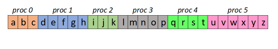
]]>Rajesh VenkatesanReading data in parallel using MPI I/O2022-10-17T10:16:20+00:002022-10-17T10:16:20+00:00https://flow-physics.github.io//hpc/2022/10/17/reading-data-in-parallel-using-mpi-i-oIn the previous post “First steps in parallel file access using MPI I/O”, we discussed how to write some simple data in parallel using MPI I/O. Here we shall read back that data in parallel. The entire code is given in my GitHub repo MPI_Notes. Essentially, we have the following text data in a file:
abcdefghijklmnopqrstuvwxyz
We will try to read this using 6 MPI processes. And we want each process to read a part of this data as shown below: (this is the same partitioning used when we wrote the data)
This partitioning is arbitrary and we could have chosen different ways to divide up the data among processes to read. Similar to the writing process, there are three approaches in MPI I/O which can be used to read this data:
Using explicit offsets
Using individual file pointers
Using shared file pointers
Using explicit offsets
As the name suggests, we need to calculate where each process should start reading its data (‘offset’) and the length of the data to be read in by that process (‘count’). So, proc 0 should read at the beginning of the file (3 characters to be read), proc 1 should start writing after 3 characters (5 characters to be read), proc 2 should start reading after 8 characters (3 characters to be read) and so on. This can be done by the following piece of code:
‘disp’ denotes the offset calculated and ‘arr_len_local’ is the count (length) of the data to read in. Once the data is read in, the MPI processes will have the following data in their ‘test_txt’ array:
While the explicit offset approach seems quite straightforward, it is preferable to use the individual file pointer method for more complex datasets and partitioning. This is discussed next.
Using individual file pointers
Since we have explained the individual file pointer method in the previous post, we shall only outline the approach here. Instead of calculating individual file pointer locations manually, we define a new global datatype to represent the data partitioning. This is done by:
In the shared file pointer approach, we specify simply the ‘count’ of the data to be read by each process and let MPI calculate the offsets for us. This can be achieved by the following code snippet:
Of course, this will come with a performance penalty as the shared file pointer is synchronized internally by MPI. The approach to use for reading/writing should be tested and its performance evaluated before deploying for production use in a software.
For demonstration purposes, we have chosen to read/write some character array in the examples here. We shall look into writing/reading general numerical data in some complex data partitioning in the next articles in this series on MPI I/O.
]]>Rajesh VenkatesanFirst steps in parallel file access using MPI I/O2022-10-13T15:08:53+00:002022-10-13T15:08:53+00:00https://flow-physics.github.io//hpc/2022/10/13/first-steps-in-parallel-file-access-using-mpi-i-oIf your code uses MPI for parallelization, then you may want to use MPI I/O for writing and reading data from files in parallel. It is common to see the use of POSIX parallel approach where each MPI process reads/writes a separate file. This approach has the following drawbacks:
Not efficiently scalable for very high number of processes
Creates a large clutter in the file system and almost unmanageable when thousands of processes are used
MPI I/O fixes these problems and provides an elegant solution for MPI applications. It is very easy to read/write data in parallel using MPI I/O if you are familiar with the basics of MPI communications (viz. point-to-point, collective). In this article, I will show you how to do this with a simple example. The entire code (written in C) can be found in full in my Github repo MPI_Notes/MPI_IO.
Parallel file writing can be thought of in the following way. Say, we have 10 people trying to write something to the same notebook. Instead of passing the notebook to them one by one, we want to tell everyone where they should start writing (e.g. the page number) their part so they can all write at the same time. Obviously, we don’t want any of them to overwrite what others have written. So we need to have the page numbers for each person calculated correctly based on:
How much would be written by others before the current person writes their part? This is called ‘displacement’
How much we expect this person to write? This is the ‘length/count of the data’
In the case of POSIX parallel I/O, we would simply be giving separate notebooks to each person and let them write whatever they want. So, we don’t have to calculate the above things. But then, it is a lot of notebooks to carry around! It may not be possible to distribute and collect back these many notebooks in a short time as well.
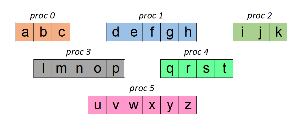
Let us assume that we have 6 MPI processes in our code. And each of them have some data in a character array as shown below:
We shall ask this data to be written to a single file. And we expect the final data to be in order of the ranks, thus listing all the alphabets in sequence. There are three ways to do this in MPI I/O:
Explicit offset
Individual file pointers
Shared file pointers
Using explicit offsets
As the name implies, we simply calculate the location where each process needs to write. This is usually specified as an ‘offset’/’displacement’ from the beginning of the file. In our example, proc 0 should write at the beginning of the file (after 0 characters), proc 1 should start writing after 3 characters (that would be written by proc 0), proc 2 should start writing after 8 characters (to take into account data from proc 0 and proc 1) and so on. Clearly, every process needs to know only where it should start writing. Additionally, we also need to inform MPI about how much data would be written.
Both this information should be supplied in the units of the datatype we are writing. In this example, the data is made of characters (these are MPI_CHAR type). The following code snippet opens/creates a file for parallel access by MPI I/O and the writes the data using the explicit offset approach collectively: (Full code here)
Once we run the program with 6 MPI processes, we will have the file “file_exp_offset.dat” written to disk. As we have written character data, we can view the contents of this file in any text editor. The file contains the following:
abcdefghijklmnopqrstuvwxyz
Using individual file pointers
When a file is opened using MPI_File_open() command, MPI creates an individual file pointer for each MPI process so that it tracks the position in file of that process. It is very similar to the file pointer in C, for example, but maintained for each MPI process separately. Note that this pointer could be in different position in the file for different processes. Using this individual file pointer, it is possible to read/write data conveniently to file in parallel. While it is possible to set the individual pointers manually per process, the most common way is to inform MPI about the global view of the data we are planning to write. Let me explain.
In our example, this can be achieved by:
// Create a MPI datatype for the global arrayMPI_Type_create_subarray(1,&total_len,&arr_len_local,&disp,MPI_ORDER_C,MPI_CHAR,&char_array_mpi);MPI_Type_commit(&char_array_mpi);
The above snippet creates a MPI datatype called ‘char_array_mpi’ which describes the global view of the data. ‘total_len’ is the total length of global data, ‘arr_len_local’ is the length of the data in the current process and ‘disp’ gives the displacement of the local data in the global array that we described earlier.
Once the global datatype is created, we inform MPI I/O by setting a ‘File View’ as follows:
‘File View’ essentially changes the way the file is accessed. MPI now knows that our read/write operations are towards reading/writing data of type ‘char_array_mpi’ and each individual process will contain only the local data for this datatype. It also additionally knows that every element we shall write is of type MPI_CHAR. This command also moves the individual (and shared) file pointer positions to the correct locations as per the global datatype (and redefines them as zero position of those pointers).
After setting the ‘File View’, we can write our character arrays to file using:
While this may seem a bit tedious, this approach can be used to write more complex datatypes and partitioning commonly used in MPI applications. Also, note that we can repeatedly write the same datatype again if needed without much additional effort. If we want to read/write a different type of data, we need to change the ‘File View’.
Using shared file pointers
One important point to note is that individual file pointers are what they claim to be, only ‘individual’. The processes do not know about how individual pointers of other processes move about. There are some situations where every MPI process needs to have a synchronized file pointer. For this purpose, MPI maintains a single shared file pointer for every MPI I/O file opened. When a read/write is done using this shared file pointer, every MPI process knows about a change in the shared file pointer position. For the sake of completeness, we shall demonstrate the collective writing of data using this approach in our example. The following code snippet writes using the shared file pointer:
Note that the displacements are calculated on the fly by MPI in this case as we are using the shared file pointer (because of the call to ‘MPI_File_write_ordered’). But this will come with a performance penalty as well.
Please go through the entire code here as it provides all the details. I have simplified a lot of things in this article but this is enough to get you started with MPI I/O. In the next article, we shall see how to read back the data in parallel.
]]>Rajesh VenkatesanParallel computing approaches for CFD2021-05-05T18:09:52+00:002021-05-05T18:09:52+00:00https://flow-physics.github.io//hpc/2021/05/05/parallel-computing-approaches-for-cfdWhen it comes to parallel computing, there are many ways to solve any complex scientific computing problem. Some are more suitable than others. The method and approach should be determined on a case by case basis with an understanding of the computational algorithm and data structures involved. In this series of articles, I will describe the different parallel computing approaches I have used for computational fluid dynamics (CFD) simulations. These provide examples of widely used approaches and I hope that they will help the reader to parallelize their scientific computing programs. I assume that the reader is familiar with the basics of MPI and OpenMP models of parallel computing.
We shall look at the following approaches:
Slab decomposition with MPI
* e.g. Direct Numerical Simulation (DNS), Poisson equation solver
Pencil decomposition with MPI
* e.g. DNS, Poisson equation solver
Solving a large ODE system in parallel - using MPI, OpenMP, Hybrid MPI+OpenMP
* e.g. vortex sheet evolution
Graph partitioning with MPI
* e.g. unstructured mesh CFD
Coupling two MPI parallel applications
The first case I will discuss is the ‘Slab decomposition’ strategy.
Slab decomposition with MPI
I used this approach in my Direct Numerical Simulation (DNS) code to simulate turbulent boundary layers. Essentially, we need to simulate the flow in a box as shown below.
And the aim is to simulate this flow using as many processors as possible. I chose the MPI (the standard for distributed parallel computing) approach. The processors work independently in this model on their data and communicate with each other when they need to exchange data/information.
In this problem, the computation needs to be performed for every point (discretized) in the rectangular box. Fortunately, all the parts of the box have almost the same amount of computation/workload. There are special treatments required for the bounding surfaces for boundary conditions. But this is very minor compared to the majority of computational workload at individual points. So, it makes sense to divide the flow domain into equal parts and distribute the parts among processors. This is critical since if one of the processors is overworked, it would create a bottleneck for other processors continuing on with their calculation. Note that the computation is inter-dependent and exchange of data is necessary (to be discussed later). The act of making sure each process handles an equal share of the computation and no bottlenecks arise due to this division of workload is called “load balancing”. In this particular case of flow in a box, it so happens that dividing the flow domain equally would lead to equal workload for each process.
So, how does one go about dividing the box domain so that the processors work efficiently together? A well known approach for such simulations is the ‘slab decomposition’ shown below.
We split the entire domain into ‘n’ slices in the x-direction, just like cutting a loaf of bread. Each slice will be given to a processor/core. The grid and variable values associated with a given part is available only in the processor owning that part. Throughout the simulation, we expect to maintain this association.
If the slices are totally independent of each other and can proceed with their part of the calculation without depending on data from neighbouring slices, then the job is literally done. But this is not usually the case. The calculations in a slice will depend on neighbouring slices which reside in another processor’s control. Particularly, it would be necessary to access at least the data from points on the neighbouring slice’s surface. The idea of ‘halo cells’ is introduced for this purpose which stores the neighbour’s data (only the required part). How this data communication is handled is very important as it will play a crucial role in overall speed of the simulation. It is possible in MPI to introduce what is known as “Cartesian topology”. This will help considerably in the ‘halo cell exchange’ of data from neighbouring processors.
Additionally, there may be parts of the simulation where it might be necessary to have the slab decomposition done in another direction instead of the original x-direction. For example, the slabs created in the z-direction is shown below.
To achieve this configuration, we have to ‘transpose’ the necessary data from the x-wise slabs to z-wise slabs. Lots of data exchange/communication is involved in this process. So, it would be wise to do this only when absolutely necessary. ‘Transposition’ should be done efficiently as well.
(to be continued…)
]]>Rajesh VenkatesanAn invitation to fluid dynamics from the oceans2020-06-27T11:01:44+00:002020-06-27T11:01:44+00:00https://flow-physics.github.io//fluid%20dynamics/movies/2020/06/27/an-invitation-to-fluid-dynamics-from-the-oceansThe last few weeks, I have been engrossed with the oceans and navigation in their vast expanse. It all started with a couple of movies I watched. The first movie “Kon-Tiki” beautifully portrays the 1947 expedition by Norwegian explorer and ethnographer Thor Heyerdahl across the south pacific, from Peru to polynesia. The remarkable thing was that he achieved this (along with some of his friends) in a balsawood raft! He was trying to establish that Incan people were the first to populate the polynesian islands. This claim is still contested today. Nevertheless, this is an extraordinary feat. They were trying to catch the south equatorial current in their raft. This made me wonder how they were relying on its presence and persistence.
Another movie I watched was “Master and Commander: The Far Side of the World” by Peter Weir. It is about a british captain (played by Russell Crowe) of a small warship trying to maniacally battle a French warship all around South America in in the atlantic and pacific oceans at the turn of the 19th century (fictional story). The thing that most impressed me was that these were both sailing ships. Once again, I started wandering the internet about how the sailors were relying on trade winds to navigate the oceans.
Being a student of fluid mechanics, I started digging deeper and found a treasure trove of books on physical oceanography. The first thing a person must appreciate when trying to study the oceans is the Earth’s rotation. This leads to the Coriolis force as we are observing Earth while moving along with its rotation. The Coriolis force plays a major role in creating the peristent ocean currents and the trade winds. Though I have had an acquaintance with geophysical fluid dynamics, it always takes a spark to make one go mad about a subject. This spark came from Henry Stommel’s great little book “Science of the Seven Seas” (freely available here). The way Stommel has introduced the oceans and its mystery to the reader is wonderful. Any high school student or undergrad picking up this elementary book would really feel what Stommel describes as “the call of the sea”. The fluid mechanics of the ocean and the atmosphere is facinating. While the fluid mechanics as a subject is quite mature with a long illustrated history, the scale of the oceans and the atmosphere leaves our computations and understanding falling short of satisfaction. Of course, this only gives impetus to the thousands of scientists working in this area to search deeper into nature. Henry Stommel was one of the great scientists in this field and his popular introduction definitely leaves a lasting impression about the subject and will inspire many to take up the oceans for their study and lifelong pursuit. I also highly recommend his more technical works (see here).
]]>Rajesh VenkatesanWhat is the Fourier transform?2020-05-24T10:28:50+00:002020-05-24T10:28:50+00:00https://flow-physics.github.io//mathematical%20physics/2020/05/24/what-is-the-fourier-transformPrevious article:1. Fourier transform for confused engineers
What is the Fourier transform, really?
For some, it is the magic of seeing everything as waves. For others, it is like holding a prism in a beam of sunlight and seeing what it contains, a rainbow of colors. For some others, it is a tool to visualize what a piece of sound recording contains and adjusting it to make it sound better.
One can even take the romanticism out of the concept and say, it converts a bunch of given numbers into another bunch. It is through doing this that many important uses of Fourier transform can be realized. And this is precisely where many miss the woods for the trees. I hope to bridge both sides of this amazing idea. Let us begin!
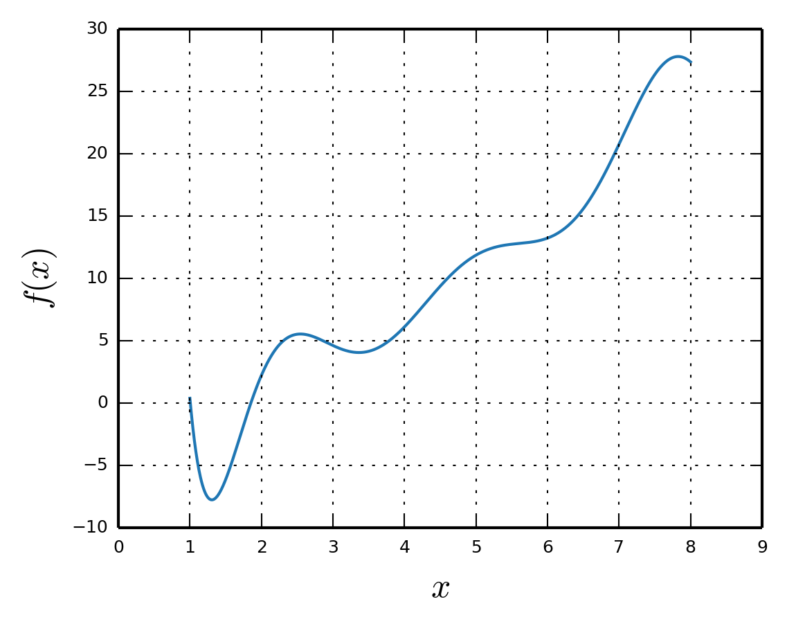
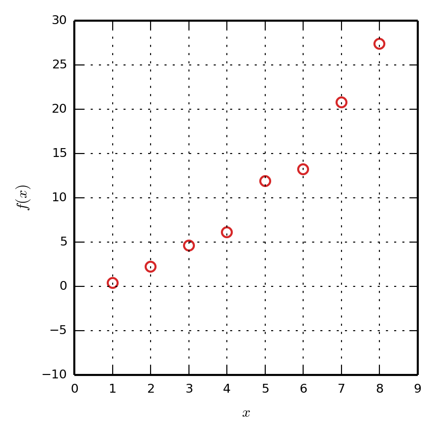
When we have a clearly defined function, as shown in the plot below, everything is straightforward.
This means that we have a known expression for how the function depends on the variable x:
\[f = f(x)\]
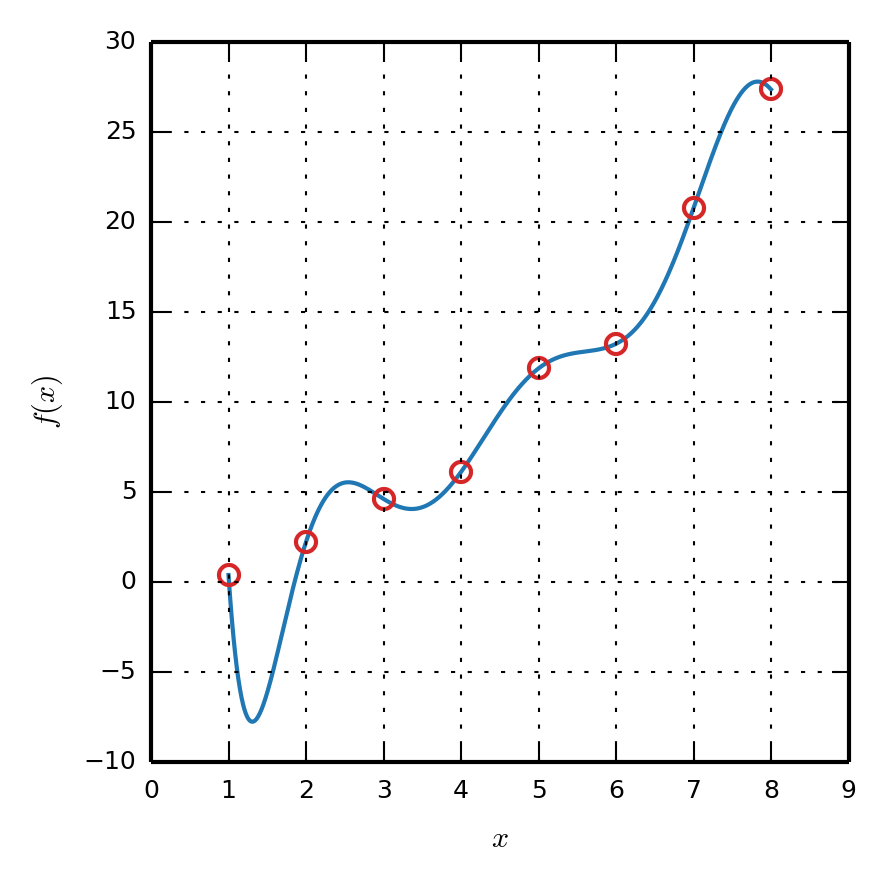
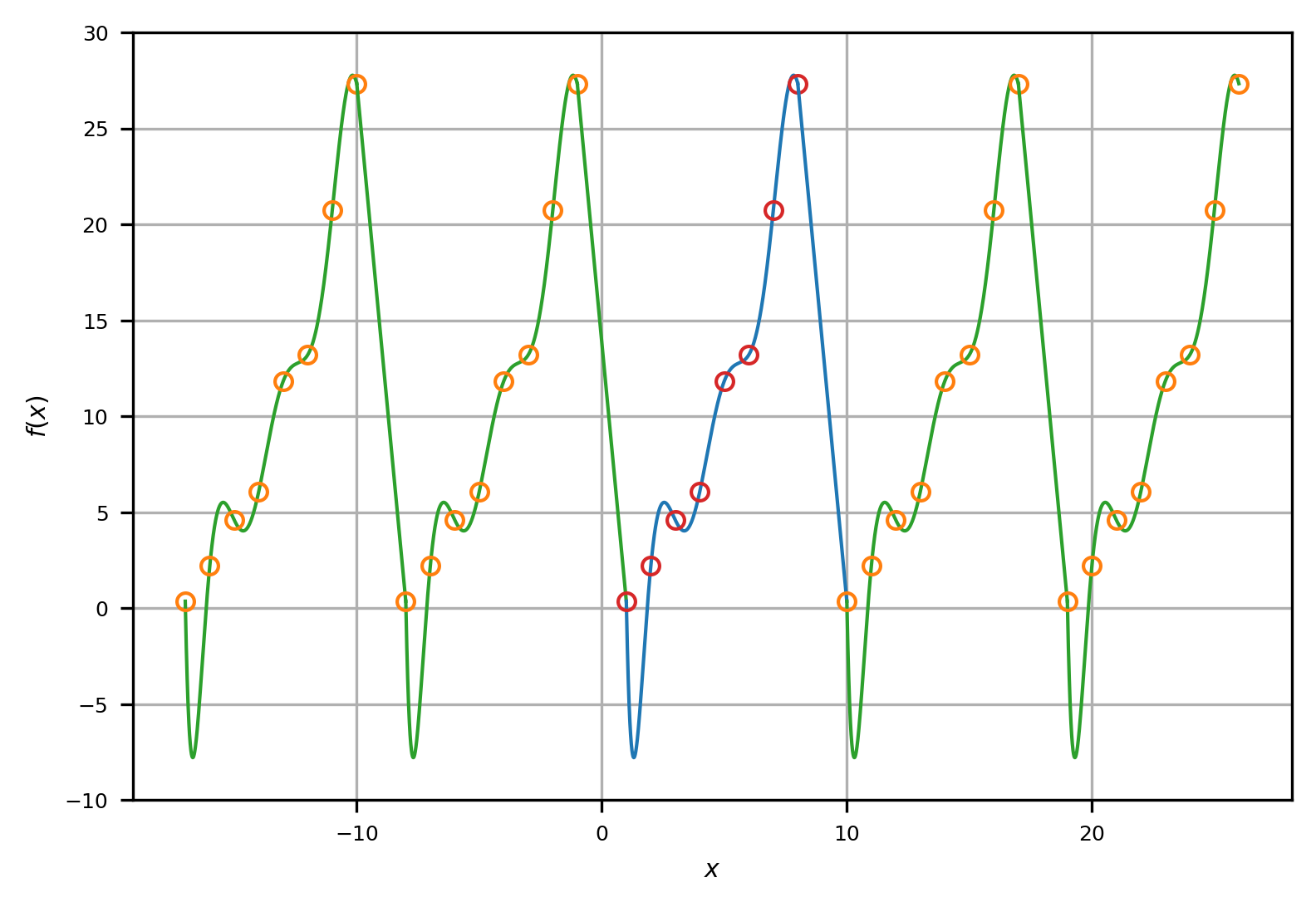
All the nice definitions of the Fourier transform become useful and if the integral is not monstrous, we would have a good looking expression for the Fourier transform of the function. Life is tricky and usually we only have some values of the function at hand. Like:
Most of the time, we just have the data points as shown by the red dots. You can imagine a function passing through the data like the blue line. But it does not matter. Now, it is just us and the red dots. The entire business of discrete Fourier transform (DFT) is to take the Fourier transform of such a bunch of data points. Before I throw some formulas at you, there are some ground rules to cover.
The universe plays the game strict and fair. If you have $N$ values in the data set, you will only get back $N$ number of values from the DFT. If you are getting anything more than $N$ values, then some of them are definitely redundant.
The most common data points are spaced (sampled) uniformly as equi-distant points in $x$. This is usually the case since most of the digital systems sample signals at a given rate. We shall always assume this to be true in our discussions. If your samples are non-uniformly spaced, you might want to look elsewhere.
The DFT models the data (and the underlying function - the blue line) using sines and cosines. Not just any sines and cosines. Some that are chosen particularly for the current dataset.
Euler’s identity is the key to everything and never lose sight of it:
\[e^{i\theta} = \cos \theta + i \sin \theta\]
With all this preamble aside, let us look at how DFT is defined for a given set of $N$ data points (like the red dots in the plot above). We will list them as:
\[f_0,f_1,f_2 . . . , f_{N-1}\]
And it is also given that these points are spaced at intervals $ \Delta x$.
Now, we shall use a trick to tell the DFT that our set of points is periodic, even though they are actually not. Imagine that the given set of points are repeated infinitely on both sides, like:
We have got the function looking like a periodic function. But what is the period of our function (the repeated pattern in the plot above)? How long does a single period span in $x$? This is easy. Take a look at the blue part of the curve above which corresponds to one period. We see that this part contains all the points $f_0,f_1,f_2 . . . , f_{N-1}$, but we also need to connect to the adjacent point (from the start of green curve). So, we actually have to include another point in our dataset (to make it periodic) which is given by $f_N = f_0$. This is important to calculate the period. Now, there are in total $N+1$ points with the number of intervals among them as $N$. The interval spacing is $\Delta x$. So, the period is,
\[L = N \Delta x \Delta s=1\]
But we usually do not include the last point $f_N$ in the dataset to avoid redundancy (since it simply repeats the $f_0$ value again). We just call our function periodic (in the sense given above) and this is enough.
Now that we got that clarified, the DFT for our data points is given by the strange looking formula:
\[F_k= \frac{1}{N}\sum\limits_{n = 0}^{N-1} f_n e^{-i 2\pi n k/N}\qquad k = -(N/2)+1,..,-2,-1,0,1,2,...,N/2\]
We need to understand what this formula says in all its glory. $F_k$’s are the Fourier coefficients and there are in total $N$ of them corresponding to as many Fourier modes. The above formula is actually $N$ similar looking formulas abbreviated into one. The symbol $k$ stands for the wavenumber/frequency associated with the Fourier mode. We will see what this all means in the next post.
P.S.: Have you noticed that the period $L$ does not even appear in this equation?! Have we wasted time in understanding the period of our function (in a strange made-up sense explained above)? NO!! You will later see that it plays a crucial role in understanding the DFT and appears explicitly in the derivative of our function if we are interested in that.
]]>Rajesh VenkatesanFourier transform for confused engineers2020-02-22T20:19:54+00:002020-02-22T20:19:54+00:00https://flow-physics.github.io//mathematical%20physics/2020/02/22/fourier-transform-for-confused-engineersIf you are an engineer, you most likely encountered one of the following situations:
Plot the power spectral density of a signal you have
Find the dominant frequency/mode in a signal
A journal paper stating, “It is obvious(?!) that this operation is straightforward to carry out in wave space”.
I have been in many such instances myself and referred several texts on Fourier analysis. There are some wonderful ones, don’t mistake me, but I have always felt that it is not straightforward to see the implications of the theory in the output of a Fourier transform function spit by a program/library in Python/Matlab. There are many equivalent ways in which the Fourier transform can be formulated, computed and interpreted. Throw the dreaded complex numbers in the mix , it is quite normal to feel lost. The feeling of not fully comprehending the idea, and yet repeatedly using it like a black box is frustrating. Having once been lost myself and now with a good grip on the means and ends of this wonderful mathematical tool, I attempt to write about this often-explained but rarely-understood method. This is mainly for my satisfaction, and if it helps someone understand this tool with a bit more of clarity, I will take that too.
This is the start of a series of posts on how to numerically compute and interpret the Fourier transform of signals/images/fields. Let’s dive right in!
]]>Rajesh VenkatesanInstalling HDF5 and CGNS in Ubuntu 18.04 LTS2019-07-21T10:29:56+00:002019-07-21T10:29:56+00:00https://flow-physics.github.io//installing%20software/2019/07/21/installing-hdf5-and-cgns-in-ubuntu-18-04-ltsIf you are a computational fluid dynamics (CFD) practitioner, at some point, you would have to use Hierarchical Data Format 5 (HDF5) and CFD General Notation System (CGNS) libraries in your programs. HDF5 format provides an advanced way of organizing any data and allows efficient access to the data. CGNS prescribes specific methods and practices to use when writing CFD simulation data into HDF5 format. You can find more info on everything about these libraries in their website. But here, I describe the way to install HDF5 & CGNS in a Ubuntu 18.04 system.
The installation procedure follows what is given in CGNS website, but with some important tweaks to get it to succeed installing in Ubuntu 18.04.
Download the CGNS source code into some directory.
Currently, this downloads CGNS 3.4.0 source code into a directory named CGNS in the present location. Although you can install HDF5 separately, and possibly a newer version from HDF5 website, I strongly advise against it. We want the CGNS library to work with our HDF5 installation. So, it is best to install the HDF5 version suggested by CGNS.
Change into the CGNS directory.
cd CGNS
There are install scripts provided in the bin folder. Three of them in fact, one to install HDF5 (./bin/install-hdf.sh), another to configure CGNS for our system (./bin/config-cgns.sh) and the last one to install the configured CGNS (./bin/build-cgns.sh). Of course, we need to do the installation in the order I have listed.
You can choose to use the install-hdf.sh script. Some options inside that script failed for me. So, instead, use the following commands:
This will download the HDF5 v1.8 into the newly created directory hdf5_1_8. Change into this directory and use the following command:
cd hdf5_1_8
./configure --enable-fortran--disable-hl--prefix=$HOME/hdf5 && make > result.txt 2>&1 && make install
Note that I am choosing to install HDF5 in the location $HOME/hdf5, you can choose any other convenient location as well. But remember, this is the location you need to link any program trying to compile with HDF5 libraries.
The installation of HDF5 will take some time, and finally it will output the HDF5 configuration installed in the system. I have configured HDF5 to include Fortran bindings as well by the flag --enable-fortran. If you only want C binidings, you can replace that by --disable-fortran.
After this, we need to configure CGNS using the ./bin/config-cgns.sh script. The default script looks like this:
Apart from some specific modifications to make it work for Ubuntu, I have also specified the CGNS installation directory as $HOME/cgns. You can change this to any other convenient location. But again, this is where the built CGNS libraries and headers will be kept. You will be required to link to this location when compiling and linking programs with CGNS.
(If you have installed the HDF5 to some location other than $HOME/hdf5, you should specify that here in the flag --with-hdf5=)
Run this configure script using:
sh ./bin/config-cgns.sh
This will configure the CGNS for your system.
Finally, install CGNS using:
sh ./bin/build-cgns.sh
That’s it. You have installed HDF5 & CGNS in your Ubuntu system at $HOME/hdf5 and $HOME/cgns respectively.
There are test codes available inside the downloaded CGNS repo at: ./CGNS/src/Test_UserGuideCode. They would have been tested during the build process as well.
If you have a program test.c which uses CGNS functions, then you would want to compile and link the program as follows:
test.out is the final executable created for the program.
Notice that we have chose not to install the utility tools for CGNS by choosing the flag --disable-cgnstools in out configure script. Enabling this fails for me. I tried to install cgnstools using various other methods as well, but it fails for me in Ubuntu 18.04.
HDFVIEW
If you want a GUI for viewing your CGNS/HDF5 files, you may want to use HDFVIEW software. Note that the hdfview available in ubuntu repositories does not work. Even the source code compilation process always fails in ubuntu. Just download the prebuilt binary for CentOS7 from the HDF website. And run the HDFView-3.1.0-Linux.sh script inside the downloaded archive to create the binary. It works properly in Ubuntu 18.04. I found this useful tip from Michael Hirsch’s blog.
]]>Rajesh VenkatesanNumerical Solution of the Falkner - Skan Equation2015-02-27T05:49:16+00:002015-02-27T05:49:16+00:00https://flow-physics.github.io//fluid%20dynamics/mathematical%20physics/2015/02/27/numerical-solution-of-the-falkner-skan-equationFalkner - Skan equation is a third order non-linear ordinary differential equation which arises in the laminar boundary layer flow past wedge-like objects. (More details here). The equation reads,
where m is a constant representing the pressure gradient parameter. Our objective is to solve this differential equation for $ f(\eta)$ , for a given value of m using the boundary conditions,
$ f’(0)=0 \quad \rightarrow \text{ no-slip condition at the wall}$
$ f’(1)=1 \, \rightarrow \text{free-stream velocity is reached at the edge of the boundary layer}$
Generally, initial value problems (IVP) are preferred for ODEs. In the case of IVP, We will be given where to start and which direction to proceed. Then we use the differential equation to progress in that direction in a step by step manner. But here we have a boundary value problem. Shooting method is used in situations where a boundary value problem has to be solved using initial value methods. The method is described as follows.
Shooting method
Guess two values for $ f’'(0)$.
Solve the FS equation using RK4 method with initial conditions $ f(0)=0, f’(0)=0, f’'(0) = Guess1$.
Solve the FS equation using RK4 method with initial conditions $ f(0)=0, f’(0)=0, f’'(0) = Guess2$.
Find out the resulting boundary value $ f’(1)$ from both these solutions.
If the boundary value $ f’(1)$ is different from the required value $ f’(1)=1$, find a better initial guess using Secant method.
Solve the FS equation by RK4 method using the new initial value guess (obtained from secant method).
Repeat the process until the required boundary value $ f’(1)$ is obtained.
A Fortran program for solving the Falkner-Skan equation implementing the above algorithm is provided below. (Click on any part of the code and use right arrow key to scroll to right).
programfalkner_skan! this program solves the Falkner-Skan equation using shooting method and fourth order Runge-Kutta method.! the FS equation is given by,! f'''+((m+1)/2)ff''+ m*(1-f'^2) = 0! m,the pressure gradient parameter, as in u_inf=u0*x^m.! boundary conditions: f(0)=0, f'(0)=0, f'(1)=1! the third order ode is converted into a system of three first order odes where the! dependent variables are f, u (=f'), v (=u'=f'').! we solve the initial value problem f(0)=0,f'(0)=0, f''(0)=guess and shoot for solutions such that f'(1)=1.implicitnoneinteger::i,j,np,niterreal,allocatable,dimension(:)::f,u,v,etareal::m,mh,re,ue,f0,u0,v0,deta,x,eps,cnu,slope,unp,unp1,vnp,vnp1real,allocatable,dimension(:)::vvel,y,vvel1real::delta_star_temp,theta_temp,deltas,thetaniter=1000! no. of iterations for the shooting methoddeta=0.001! non-dimensional spacing in the wall-normal directionnp=8001! no. of points in the wall-normal directioneps=1.0e-16! error margin used in shooting method iterationm=0.0! falkner-skan pressure gradient parametermh=0.5*(m+1.0)allocate(f(np),u(np),v(np),eta(np),vvel(np),vvel1(np),y(np))! form the grid in the wall-normal directioneta(1)=0.0doj=2,npeta(j)=eta(j-1)+detaenddo! initial values set 1f0=0.0u0=0.0v0=0.335callrk4_fs(f,u,v,deta,mh,m,np,f0,u0,v0)vnp=v(1)unp=u(np)! initial values set 2f0=0.0u0=0.0v0=0.33callrk4_fs(f,u,v,deta,mh,m,np,f0,u0,v0)vnp1=v(1)unp1=u(np)! loop for the shooting method ********************************************************************doi=1,niterif(abs(unp1-1.0).ge.eps)thenslope=(vnp1-vnp)/(unp1-unp)v0=vnp1+slope*(1.0-unp1)unp=unp1vnp=vnp1callrk4_fs(f,u,v,deta,mh,m,np,f0,u0,v0)vnp1=v(1)unp1=u(np)elsewrite(*,*)'iteration converged'write(*,*)'v(1)=',v(1)exitendifif(i.eq.niter)thenwrite(*,*)'maximum number of iterations reached'endifenddo! end of shooting method **************************************************************************doj=1,npwrite(38,*)eta(j),f(j),u(j),v(j)! these are transformed variables - input for box methodenddo! calculation of normal velocity component profilex=0.1u0=1.0ue=u0*(x**m)cnu=15.0e-06re=ue*x/cnudoj=1,npy(j)=eta(j)*sqrt(cnu*x/ue)! distance from the wall in metersvvel(j)=-((m-1.0)*eta(j)*u(j)+(m+1.0)*f(j))*(0.5/sqrt(re))! vvel=v/u_infwrite(48,*)eta(j),u(j),vvel(j),y(j),u(j)*ue,vvel(j)*sqrt(re)enddo! calculation of boundary layer parameterstheta_temp=0.0delta_star_temp=0.0doi=1,(np-1)theta_temp=theta_temp+0.5*(eta(i+1)-eta(i))*(u(i+1)*(1.0-u(i+1))+u(i)*(1.0-u(i)))delta_star_temp=delta_star_temp+0.5*(eta(i+1)-eta(i))*((1.0-u(i+1))+(1.0-u(i)))enddodeltas=delta_star_temp*x/sqrt(re)theta=theta_temp*x/sqrt(re)write(*,*)'************************************************************************'write(*,*)'Solution of the Falkner-Skan equation'write(*,*)'************************************************************************'write(*,'(a,f8.5)')'pressure gradient parameter, m=',mwrite(*,'(a,f8.5,a)')'distance from the leading edge, x=',x,' m'write(*,'(a,f8.2)')'Re = u_inf*x/cnu = ',rewrite(*,'(a,f8.5,a)')'displacement thickness, delta*=',deltas,' m'write(*,'(a,f8.5,a)')'momentum thickness, theta=',theta,' m'write(*,*)'************************************************************************'callsystem('gnuplot -p FS.plt')returnendprogramfalkner_skansubroutinerk4_fs(f,u,v,deta,mh,m,np,f0,u0,v0)! subroutine for solving a system of three first order odes with fourth order Runge-Kutta method! f0,u0,v0 are the initial values! f,u,v arrays give the solution! initial values are propagated to np steps using step spacing deta.integer::jreal::kf(4),ku(4),kv(4)real,intent(in)::m,mh,deta,f0,u0,v0integer,intent(in)::npreal::f(np),u(np),v(np)f(1)=f0u(1)=u0v(1)=v0doj=2,npku(1)=v(j-1)kf(1)=u(j-1)kv(1)=-mh*f(j-1)*v(j-1)-m*(1.0-u(j-1)*u(j-1))ku(2)=v(j-1)+0.5*kv(1)*detakf(2)=u(j-1)+0.5*ku(1)*detakv(2)=-mh*(f(j-1)+0.5*kf(1)*deta)*(v(j-1)+0.5*kv(1)*deta)-m*(1.0-(u(j-1)+0.5*ku(1)*deta)**2)ku(3)=v(j-1)+0.5*kv(2)*detakf(3)=u(j-1)+0.5*ku(2)*detakv(3)=-mh*(f(j-1)+0.5*kf(2)*deta)*(v(j-1)+0.5*kv(2)*deta)-m*(1.0-(u(j-1)+0.5*ku(2)*deta)**2)ku(4)=v(j-1)+kv(3)*detakf(4)=u(j-1)+ku(3)*detakv(4)=-mh*(f(j-1)+kf(3)*deta)*(v(j-1)+kv(3)*deta)-m*(1.0-(u(j-1)+ku(3)*deta)**2)f(j)=f(j-1)+(1.0/6.0)*deta*(kf(1)+2.0*kf(2)+2.0*kf(3)+kf(4))u(j)=u(j-1)+(1.0/6.0)*deta*(ku(1)+2.0*ku(2)+2.0*ku(3)+ku(4))v(j)=v(j-1)+(1.0/6.0)*deta*(kv(1)+2.0*kv(2)+2.0*kv(3)+kv(4))enddoendsubroutinerk4_fs
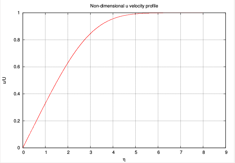
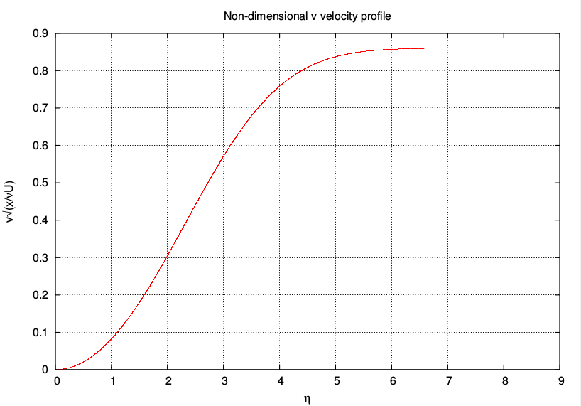
Line 114 in the above code calls the gnuplot program FS.plt to plot the solution. The most relevant plots for fluid dynamics in this problem are the streamwise velocity profile $ f’(\eta)$ and the wall-normal velocity profile given by,
Sample results for the case m=0 (Blasius boundary layer) are shown below.
]]>Rajesh VenkatesanWhy are sound waves longitudinal?2014-10-12T06:00:48+00:002014-10-12T06:00:48+00:00https://flow-physics.github.io//mathematical%20physics/2014/10/12/why-are-sound-waves-longitudinal“Give me some example for waves in nature! “
“Sound is a wave.. Light is a wave.. Of course we see water waves.. “
Thats the usual answer we think about when asked that question. Moreover, we are told that sound waves are longitudinal waves (compression waves) and light waves are transverse waves. But we do not often ask the question ‘Why?’. Why are sound waves longitudinal?. I give a short answer and a lengthy one.
Short Answer
Both light propagation and sound propagation (in air or water) are governed by the same wave equation. But in case of a light wave or traveling waves on a string, the variable governed by the wave equation is the disturbance itself. Thus leading to a transverse wave. In the case of a sound wave, the variable governed by the wave equation is the velocity potential $\phi$. This is related to the disturbance velocity in the following way,
\[\vec{V}=\nabla \phi\]
And from vector analysis, it is easy to show that the gradient vector $ \nabla \phi$ is perpendicular to constant lines of the original field $ \phi$. Hence, even though $ \phi$ propagates like a transverse wave, the disturbance velocity $ \vec{V}$ propagates like a longitudinal wave.
Long Answer
Waves are everywhere around us. In simple terms, a wave is a disturbance propagating through a medium (say, air or water). Most wave phenomenon we see in nature are governed by the so-called wave equation,
The solution to the above equation is any (good!) function traveling in the x-direction with speed c. Formally written as $ \psi=f(x\pm ct)$. For example, in the case of a ripple in a pond, a change in the height of the water plays the role of the disturbance. This change propagates through the pond from the source that created the disturbance. In this case, $ \psi $ is the displacement of water from the undisturbed level.
Similarly, for a light wave, the thing that changes is the electromagnetic field. And this change is propagated through space. There are two types of waves. Longitudinal waves and transverse waves. In the example given above, the change in the water level is propagating outwards throughout the pond. But the change itself makes the water go either up/down at a given location. Thus we say, the wave propagates in one direction and the displacement of the medium is at right angles to that direction. This kind of wave is called a transverse wave. An illustration of a transverse wave is given below: (taken from Wikipedia)
On the other hand, we have longitudinal waves where the displacement of the medium occurs in the same direction as that of wave propagation. This is illustrated in the following image: (taken from Wikipedia)
When sound propagates from left to right, the air molecules are compressed and rarefied just like the vertical grid lines in the above figure. During sound propagation in the x-direction, the velocity potential obeys the wave equation.
(This equation is derived from the Navier-Stokes equation after linearization and some other assumptions).
The solution to the above equation is given as,
\[\phi=f(x\pm ct)\]
From this solution and the definition of the velocity potential ($ \vec{V}=\nabla\phi$), we can find the disturbance velocity field as,
\[u=f'(x \pm ct)\]
\[v=0\]
\[w=0\]
Thus we see that the transverse wave of $ \phi$ in the x-direction leads to a disturbance velocity involving only the x-component velocity u. So the air/water molecules are displaced in the same direction as the direction of propagation.
Note
Sound waves propagate as longitudinal waves in fluid media. In solids, however, they travel both as longitudinal and transverse waves.